Hierarchical alignment between cortical representations and vision-language latent spaces
N. A. Adarsh Pritam1 Jeba Shiney O1Sanyam Jain2,3
1Alliance School of Advanced Computing, Alliance University, India
2Department of Dentistry and Oral Health, Aarhus University, Denmark
3Department of Computer Science and Communication, Østfold University College, Norway
Same brain data, same frozen image generator. Only the map from cortex to latent space changes.
1The question
Brain-to-image systems keep getting heavier generators. We left the generator alone and
asked what kind of map the brain-to-latent interface actually is.
A person lies in a 7 tesla scanner and looks at photographs. The scanner measures blood oxygenation
across thousands of voxels of visual cortex. To turn that back into a picture, current methods learn a map
from voxels into the latent space of a pretrained image generator, and let the generator do the drawing.
Almost everyone uses ridge regression for that map, a single matrix, and spends their effort on the
generator instead.
That assumes cortex relates to a generative model's latents the same way everywhere. We think it does not.
Early visual cortex carries something close to a picture: edges, layout, contrast. Higher visual areas carry
what the scene is: a giraffe, a kitchen, a person on a surfboard. Those two things live in different
parts of a diffusion model too, one in the autoencoder latent, one in the CLIP conditioning vector.
If the brain is organised as a hierarchy, then the map out of it should not be one map.
It should be near-linear at the bottom and clearly nonlinear at the top.
The panel below is that hypothesis with the measured numbers attached. Pick a region of visual cortex and
see which part of the generator it feeds, and how much a nonlinear decoder buys you there.
Where does a nonlinear decoder pay off?
Click a region on the cortex, or use the two buttons.
Early visual cortex, V1 to V3
Almost linear already.
Ridge regression gets most of the way to the diffusion latent. Adding depth and
nonlinearity to the decoder helps a little, and then stops helping.
Ridge regression0.239
Residual MLP (ours)0.300
+0.06
correlation with the true latent, subj01.
Correlation between predicted and true latents on the 982 shared test images. The routing of
early cortex to z and ventral cortex to c follows the region split used by Takagi and
Nishimoto, so the only thing we change is the decoder.
Not one map
The interface from cortex to latent space is near-linear for structure and strongly nonlinear for
meaning. One decoder family for both is the wrong default.
Only the interface
No new generator, no extra conditioning, no fine-tuning. Changing the map alone beats much heavier
pipelines on every semantic metric we report.
Latents, not pixels
An expressive decoder drifts off the generator's own distribution. Semantics improve, texture does
not. Accurate latents are necessary but not sufficient.
2How a picture comes back out
Five stages, from a photograph on a screen to a photograph rebuilt from blood flow.
Only stage three is trained.
The reconstruction pipeline
Step through it, or click a stage.
A photograph on a screen
Each of the four participants viewed roughly 10,000 natural photographs from MS COCO
over 30 to 40 scanning sessions. 982 images were shown to everyone, and those are held out for testing.
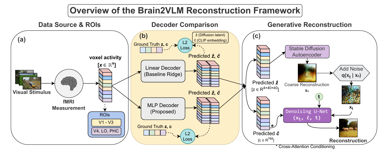
The same pipeline as it appears in the paper. (a) Voxels are taken from early
(V1–V3) and ventral (V4, LO, PHC) regions. (b) Ridge and the residual MLP are trained with an
ℓ2 loss to predict z and c. (c) The predicted z is decoded to a
coarse image, re-noised, then denoised by a U-Net conditioned on the predicted c through
cross-attention. Nothing inside the generator is trained.
The decoder itself is deliberately plain
An input projection to 2048 units, then N residual blocks of linear, GELU, LayerNorm and dropout,
then a linear output projection. Mean squared error against the true latent. The same hyperparameters are
used for all four subjects. The point was never a clever architecture; it was to have enough expressivity
to expose the difference between the two streams.
Residual MLP decoder. Drawn with N = 2 blocks; depth is varied in the
ablations below.
3What comes back
Fourteen held-out photographs from subj01. Drag the divider to swap between the linear
baseline and our decoder on the same brain data.
Reconstruction explorer
Pick a stimulus below, then drag across the image. Arrow keys work too.
Objects in this photo: giraffe
Both reconstructions come from the same fMRI recording and the same frozen Stable
Diffusion. The only difference is how the voxels were mapped into z and c.
Seen
LinearBrain2VLM
↔
Object identity is recovered far more often. Texture and fine
detail are not.
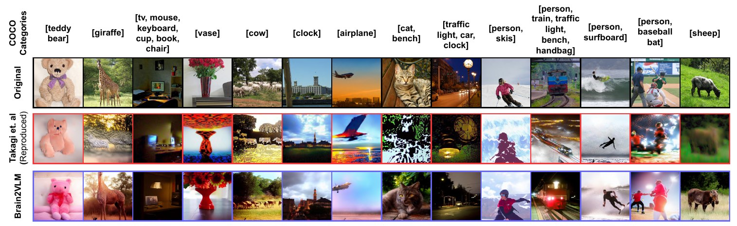
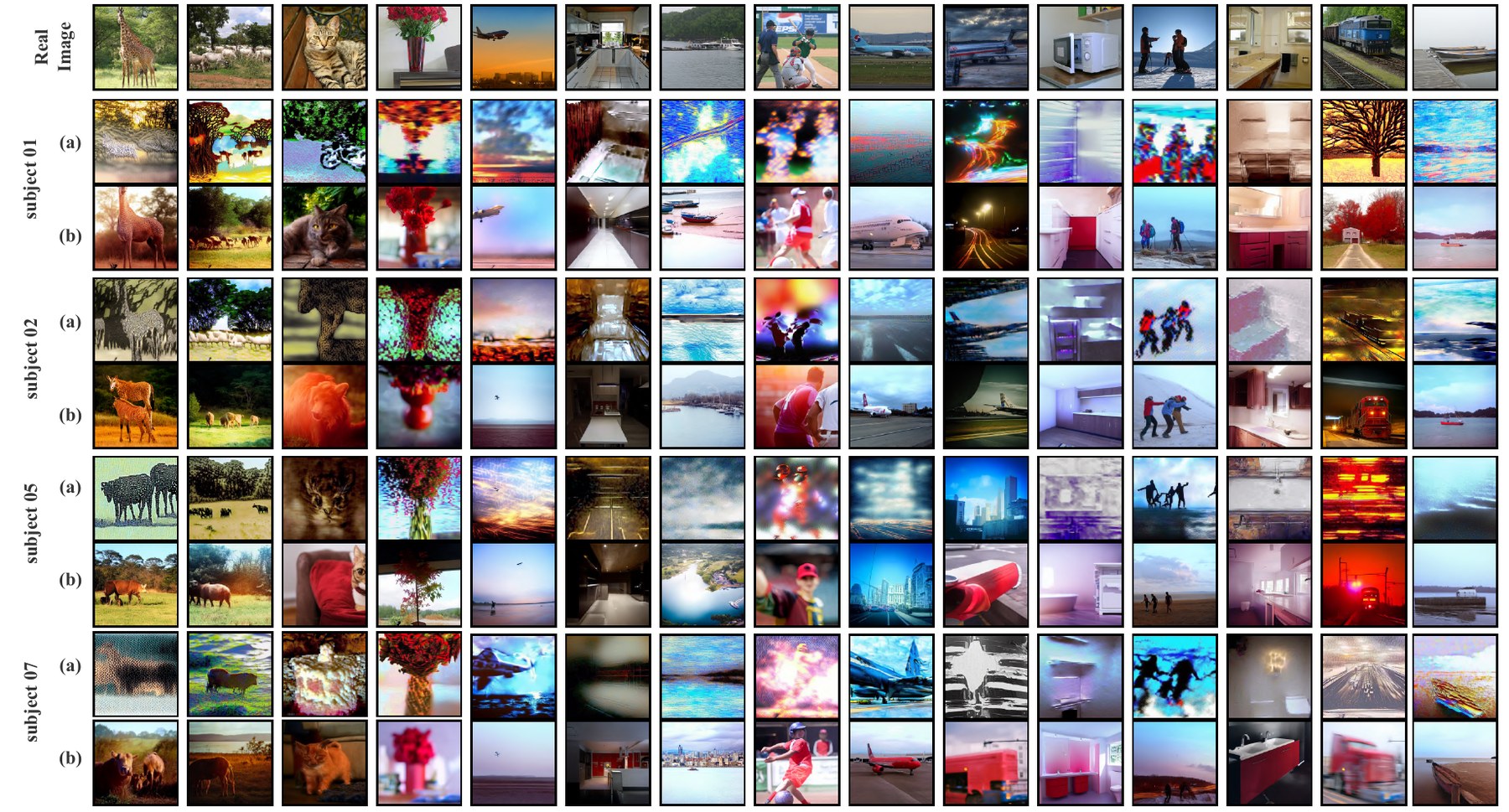
All fourteen, as printed. Top row, the photographs. Middle, reconstructions from linear
decoders. Bottom, reconstructions from our nonlinear decoders. Both recover coarse spatial structure;
the nonlinear decoder recovers recognisable categories more often.
4How much decoder do you need?
Depth, width and training data, measured separately for the structural latent and the
semantic one. The two targets behave nothing alike.
Ablation curves, subj01
Hover a point for its value.
Target
Vary
residual MLPridge baseline
Depth saturates after about two blocks and width after 2048 units, but accuracy is still climbing with
the amount of training data at the point where NSD runs out. Decoding is still data-limited, which is a
more useful thing to know than another point of correlation.
Best configuration per ablation, against
the ridge baseline. All differences are significant at p < 0.01, paired
t-test across stimuli.
Target
Ablation
Best value
Mean correlation
Std
Gain over ridge
diffusion z
depth
0 blocks
0.2959
0.0036
+0.0569
diffusion z
width
512
0.3002
0.0037
+0.0612
diffusion z
data fraction
1.0
0.2843
0.0027
+0.0453
CLIP c
depth
6 blocks
0.7819
0.0008
+0.4779
CLIP c
width
2048
0.7761
0.0012
+0.4721
CLIP c
data fraction
1.0
0.7761
0.0012
+0.4721
5Where the predictions land
Being close on average is not the same as living in the right neighbourhood. These are the
982 test predictions projected onto their first two principal components.
Predicted latents against the real ones
Toggle a cloud on or off in the legend.
Latent space
For CLIP, the linear predictions sit in their own cluster, well away from the true embeddings; the MLP
predictions land on top of them. For the diffusion latent, all three clouds already overlap, and the MLP
moves things slightly in the wrong direction. Maximum mean discrepancy says the same thing in one number.
Comparison
Latent
MMD, lower is better
true z vs linear
diffusion z
0.1213 ± 0.0018
true z vs MLP
diffusion z
0.1327 ± 0.0019
true c vs linear
CLIP c
0.3585 ± 0.0016
true c vs MLP
CLIP c
0.0424 ± 0.0004
linear vs MLP
diffusion z
0.0190 ± 0.0007
linear vs MLP
CLIP c
0.3892 ± 0.0004
A decoder can be more accurate and less compatible with the generator at the same time.
That is the tension this work puts a number on.
Correlation with the true latent rewards getting the average right. The generator cares about something
else: whether the vector you hand it looks like the vectors it was trained to condition on. For CLIP those
two goals agree, and both improve. For the diffusion latent they come apart, which is the cleanest
explanation we have for why semantic scores jump while texture does not.
6Four subjects, same story
Individual brains differ in signal quality and cortical layout. The direction of the effect
does not.
Reconstruction quality per subject
Switch participants to compare.
Participant
linear ridgeBrain2VLM
Against published pipelines
BrainDiffuser adds a VDVAE initialiser and dual-guided diffusion. MindLDM adds masked autoencoder
features, CLIP alignment, depth reconstruction and ControlNet guidance. Both keep a regression at the
brain-to-latent interface. We changed only that interface.
Metric
BrainDiffuser
MindLDM
Takagi et al.
Brain2VLM
Low-level fidelity
PixCorr, higher better
0.294
0.119
—
0.36
SSIM, higher better
0.406
0.328
—
0.31
LPIPS, lower better
—
—
—
0.69
AlexNet(5)
87%
92%
83%
92%
CLIP(6)
—
—
—
71%
DINOv2(6)
—
—
—
69%
High-level semantics
AlexNet
—
—
—
92%
CLIP
63%
83%
77%
85%
DINO
—
—
—
92%
Inception
66%
81%
76%
89%
Retrieval
top-1
—
—
—
4%
top-10
—
—
—
23%
Where on the cortex the gain lives
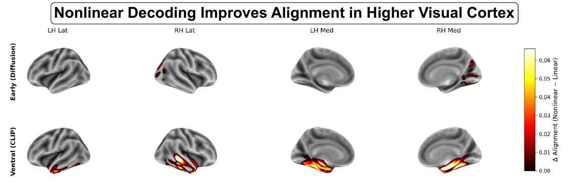
Plotting the change in alignment, nonlinear minus linear, straight onto the cortical surface gives the
hypothesis its most direct test. Early areas barely light up. The ventral stream lights up along its whole
length.
Change in alignment projected onto the cortical surface, subj01. Top row, early visual
cortex predicting the diffusion latent: sparse and weak. Bottom row, ventral cortex predicting CLIP:
strong and spatially coherent along the stream.All four participants. For each subject, the first row is the linear ridge decoder and
the second is ours. Absolute quality varies between people; the direction of the difference does not.
7What this does not settle
Four participants from one dataset is a narrow base, and every decoder here is trained within a single
subject. Cross-subject decoding and a second dataset are the obvious next tests.
The decoder never models the distribution it is predicting into, only the mean squared error to a target.
A distribution-aware loss, or a diffusion prior over latents, would let us keep the accuracy without
sliding off the generator's manifold. That is the experiment we most want to run next.
And a residual MLP is a blunt instrument for showing that a mapping is nonlinear. It shows the gap exists.
A transformer or a multimodal decoder would say more about the shape of it.
One honest caveat about reading these reconstructions: a diffusion model always produces a
plausible photograph, whether or not the brain supplied the evidence for it. Category-level metrics and the
cortical maps are what carry the claim here, not any single pretty image.
8Cite this work
@article{Pritam2026Brain2VLM,
  author    = {Pritam, N A Adarsh and O, Jeba Shiney and Jain, Sanyam},
  title     = {Brain2VLM: Hierarchical Alignment Between Cortical Representations
               and Vision-Language Latent Spaces},
  journal   = {bioRxiv},
  year      = {2026},
  doi       = {10.64898/2026.04.23.720313},
  elocation-id = {2026.04.23.720313},
  publisher = {Cold Spring Harbor Laboratory},
  url       = {https://www.biorxiv.org/content/early/2026/04/23/2026.04.23.720313}
}